Corresponding GitHub page.
To learn a bit about machine-learning methods for classifying images, I implemented several standard classifiers, namely k-Nearest-Neighbours (kNN), Logistic Regression, and Fully-Connected and Convolutional Artificial Neural Networks, and applied these classifiers to a simple problem.
Some of the prototype images above are deliberately close to each other. For example, the only difference between Circle III and Circle IV is a small disc in the center, and Pentagon and Hexagon are beginning to resemble a Circle, if a classifier cannot distinguish between rounded and straight edges (or detect corners). The card suits are examples of more complex shapes with features that aren't linear or circular.
The system is to be trained on simulated data that is generated by applying affine transformations to the above sixteen shapes (this is described in more detail below).
During test time, there are two main sources of test shapes:Of the two, user-generated input is much more challenging for the classifier, because the distribution of test shapes generated by the user over time can be quite far from the training distribution.
The results for how well each of the classifiers does on computer-generated input are described below. As for user-generated input, the reader may have a bit of fun playing around with the following applet that implements the classifiers.
The prototype shapes are represented as sets of linear, quadratic or, in some cases, cubic inequalities (that is, as real semialgebraic varieties!). To generate a training set, as many random linear transformations (four floats making up a 2x2 matrix) as needed are generated, and the inequalities that define the shape are pulled back by these linear transformations. Then, if possible, the shape is translated by a random translation chosen uniformly from the collection of all translations that do not bring the shape out of bounds of the original 128x128 image.
For testing the classifiers, I decided on three different distributions for the affine transformations, resulting in, roughly speaking, low, medium, and high levels of deformation. Specifically, the distributions are as follows.
|
The entries of the affine transformation are labeled as \( \begin{pmatrix} diag & off \\ off & diag \end{pmatrix} + \begin{pmatrix} trans \\ trans \end{pmatrix} \) |
|
Here \(N(\mu, \sigma^2)\) denotes the normal distribution with mean \(\mu\) and variance \(\sigma^2\). The elements \(trans\) of the translation are drawn from a uniform distribution over the intervals in x- and y- coordinates that keep the shape in bounds.
Here are links to several pages containing images drawn from data sets of the above three deformation types (the sets below contain several hundred images each, to lighten the memory requirements; a typical training set is much larger):
| Low deformation | 1 | 2 | 3 | 4 | 5 |
| Med deformation | 1 | 2 | 3 | 4 | 5 |
| High deformation | 1 | 2 | 3 | 4 | 5 |
The pages below display examples of test images, their closest neighbours, and the resulting classification, for data sets of various sizes and deformation levels. The classifier does fairly well for low-deformation examples, but less so with medium-deformation and especially high-deformation ones.
| Example kNN classifications: | |||
|---|---|---|---|
| 32768 examples in data set | Low | Med | High |
| 16384 examples in data set | Low | Med | High |
| 8192 examples in data set | Low | Med | High |
| 4096 examples in data set | Low | Med | High |
| 2048 examples in data set | Low | Med | High |
| 1024 examples in data set | Low | Med | High |
|
Low deformation |
Medium deformation |
The performance seems to decrease with increasing \(k\), with the best performance obtained with \(k=1\). This is in line with how kNN performs on MNIST, which is another image classification task of similar difficulty (handwritten digit recognition).
Interestingly, in the range of data set sizes I experimented with, the proportion of images that are classified correctly by kNN seems to depend logarithmically on the data set size, though it stops being so near the boundaries of the data set sizes I have seen. The following plots are obtained by averaging the results of kNN over twelve different data sets of indicated size (once again, the shaded background indicates a single standard deviation from the mean):
| Legend: Yellow: Low deformation
Blue: Med deformation
Purple: High deformation
|
Let \(X = (X_1, \dots, X_N)\) be an input, and \(Y\) the true class of \(X\), with \(Y\) taking values in the set \(\{1,2,\dots,C\}\) of possible classes. The Softmax classifier approximates the conditional probabilities \(P(Y = y | X = x)\) using a collection \( T = \{(x_1,y_1), (x_2,y_2), \dots, (x_K,y_K)\}\) of training examples. After the conditional probabilities have been approximated, their values can be used for classification: given a new input, the class of the input is taken to be the class that has the highest (approximated value of the) conditional probability.
Softmax approximates the conditional probabilities using a variant of a linear model. For convenience, add an additional coordinate \(X_0 = 1\) to the beginning of every input vector (so that the input vector now has the form \(X = (1, X_1, \dots, X_N)\)). Then, the model used for softmax takes the form $$ \begin{align*} \log P(Y = 1 | X = x) &\propto \langle \theta_1, x \rangle = \theta_{10} + \theta_{11}x_1 + \cdots + \theta_{1N}x_N \\ &\vdots \\ \log P(Y = C | X = x) &\propto \langle \theta_C, x \rangle = \theta_{C,0} + \theta_{C,1} x_1 + \cdots + \theta_{C,N} x_N \\ \end{align*} $$ Here, \(\theta_1, \dots, \theta_{C}\) are vectors in \(\mathbf{R}^{N+1}\), \(\langle a,b\rangle = a^T b\) denotes the usual dot product, and the \(\propto\) symbol denotes that the expressions on the two sides the symbol differ by a multiplicative constant. The collection of parameters \( \theta = \{\theta_1, \dots, \theta_{C}\}\) is to be fit using the training data. Because \(\sum_c P(Y=c | X = x) = 1\), the model actually has fewer degrees of freedom than may appear, and it is possible to reduce the number of parameter vectors down to \(C-1\) by fixing one of the vectors. (This is a bit more efficient to train, because it has fewer parameters, but the resulting formulation has slightly less symmetry, so I prefer not to use it here.)
Computing the proportionality constant, the model above is equivalent to $$ \begin{align*} P(Y = 1 | X = x) &= \frac{\exp(\langle \theta_1, x\rangle)}{\sum_{c=1}^{C} \exp(\langle \theta_c, x \rangle)} \\ &\vdots \\ P(Y = C | X = x) &= \frac{\exp(\langle \theta_C, x\rangle}{\sum_{c=1}^{C} \exp(\langle \theta_c, x \rangle)} \\ \end{align*} $$
A standard way of fitting the parameters \(\theta\) is using the method of maximum likelyhood. Given a labelled input \((x,y)\), with \(y\) being the true class of \(x\), the log-likelyhood of \(y\) being the class of \(x\) is given by
$$ LL(y|x, \theta) = \log P(Y = y | X = x, \theta) = \langle \theta_y, x \rangle - \log\left( \sum_{c=1}^C \exp(\langle \theta_c, x \rangle) \right) $$ We estimate \(\theta\) by the collection of parameters that maximizes the likelyhood. The derivative of the log-likelyhood with respect to the parameter \(\theta_{cn}\) (here \(c \in \{1,2,\dots,C\}\) and \(n \in \{0,1,2,\dots,N\}\)) is given by $$ \begin{align*} \frac{\partial LL(y|x, \theta)}{\partial \theta_{cn}} &= \left( 1_{y = c} - \frac{\exp(\langle \theta_c, x\rangle)}{\sum_{c' = 1}^C \exp(\langle \theta_{c'}, x\rangle)} \right) x_n \\ &= \left( 1_{y=c} - LL(y|x,\theta) \right) x_n \end{align*} $$Taking the negative of the log-likelyhood as the loss function, the set of parameters \(\theta\) that maximize the likelyhood of \(y\) given \(x\) may be iteratively approximated using gradient descent. Namely, let \(T = \{(x_1, y_1), \dots, (x_K, y_K)\}\) be a labelled training set. Drawing a minibatch \(B\) from \(T\), we get the average loss $$ \operatorname{Avg.Loss}(B, \theta) = \frac{1}{\left|B\right|} \sum_{(x_b,y_b) \in B} \left(-LL(y_b | x_b, \theta) \right) $$ Initializing the parameters \(\theta\) with some small random values \(\theta^{(0)}\), we obtain a sequence of approximations \( \theta^{(0)}, \theta^{(1)}, \theta^{(2)}, \dots\) according to the rule $$ \theta^{(k+1)} = \theta^{(k)} - \alpha^{(k)} \operatorname{grad}_{\theta^{(k)}} \left( \operatorname{Avg.Loss}(B^{(k)}, \theta^{(k)}) \right) $$ where \(\alpha^{(k)}\) is a sequence of hyperparameters usually called the learning rates. In coordinates, \(\theta\) is updated according to $$ \theta^{(k+1)}_{cn} \longleftarrow \theta^{(k)}_{cn} - \frac{\alpha^{(k)}}{\left| B^{(k)} \right|} \sum_{(x_b,y_b) \in B^{(k)}} -\left( \left( 1_{c = y_b} - \frac{\exp(\langle \theta^{(k)}_c, x_b\rangle)} {\sum_{c'=1}^C \exp(\langle \theta^{(k)}_{c'}, x_b \rangle)} \right) (x_b)_n \right) $$
To combat overfitting, we can add a regularization term to the loss function. A frequent choice is \(L^2\) regularization, which adds the term \( \displaystyle \frac{\lambda}{2} \sum_{c,n} \theta^2_{c,n} \) to the loss function, where \(\lambda\) is an additional hyperparameter of the model.
The gradient descent update then becomes $$ \theta^{(k+1)}_{cn} \longleftarrow \theta^{(k)}_{cn} - \alpha^{(k)} \left[ \frac{-1}{\left| B^{(k)}\right|} \sum_{(x_b,y_b) \in B^{(k)}} \left( \left( 1_{c = y_b} - \frac{\exp(\langle \theta^{(k)}_c, x_b\rangle)} {\sum_{c'=1}^C \exp(\langle \theta^{(k)}_{c'}, x_b \rangle)} \right) (x_b)_n \right) + \lambda^{(k)} \theta_{cn} \right] $$
The simplest choice of input features for our problem is simply the collection of 128x128 input pixels. With only pixels as input, and with no additional pre-processing, Softmax does not perform well on this problem. There are sufficiently many parameters that Softmax can overfit a data set of any deformation type, but the testing accuracy is quite low, even if the shapes are not deformed and only translated.
The following plots were all obtained with a training set size of 32,768, \(\alpha = 0.01,\ \lambda=0.0005\) and a minibatch size of 32. The blue curve represents training data accuracy, and the green curve representes test data accuracy.
|
No deformation (but with translation) |
Low deformation |
Med deformation |
High deformation |
After a moment of reflection, the poor performance of Softmax, if only the image pixels are provided as input, is not surprising. For each shape, each trained parameter represents the influence of a single pixel of the input image on the class (with the exception of the bias term). However, at the level of a single pixel, it is impossible to tell whether or not a given image is a particular shape, say a triangle, because for each pixel there exist both valid triangles that do contain the pixel, and valid triangles that do not.
A nice feature of Softmax is that the parameters it fits are often at least somewhat interpretable. If we do not deform the prototype images, the parameters obtained by gradient descent can be visualized as follows: here, the shade of each pixel is proportional to the distance of the parameter corresponding to that pixel from the minumum parameter, with the smallest parameter being black and the largest parameter being white:
There are some interesting patterns here. The small disc in the middle that distinguishes between Circle III and Circle IV gets by far the largest (or smallest parameter), the polygons have a shaded circle in the middle and the corners tend to be highlighted. The Rhombuses have shaded interiors.
For a low deformation training set, the parameters are nearly indistinguishable from noise, except at the corners, which is forced by the requirement that the training shapes do not pass out of bounds:
It is encouraging, however, how nicely Softmax works for finding the features in the sixteen image prototypes when trained on non-deformed data (in particular, the parameters seem to focus on many of the important parts of the images, such as interiors, edges, curves, and so on). One way forward is to increase the number, variety or quality of the features that are provided as input to Softmax; the pixels alone are not good enough to separate the image classes (when the images are deformed). There are two main approaches for doing this: features can be manually engineered, or can be found in an automated way (or learned). Manually-engineering features requires deeper insight into the problem, but is laborious and often task-specific. The family of automated feature-extractors (this is one point of view on them) that do best on modern benchmarks are artificial neural networks.
Another approach is to pre-process the data. Clearly, for the current problem, each image can be returned back to one of the sixteen prototypes by an inverse affine transformation, and softmax quickly trains to classify those sixteen images perfectly. For hand-drawn data, one can try to find the bounding box of the drawn shape and deform it so that the bounding box is centered and fills the entire 128x128 frame.
A series of well-known results of George Cybenko (and others) show that large fully-connected neural networks can represent arbitrary continuous functions with an arbitrarily good accuracy (as long as the number of nodes is allowed to depend on the accuracy). This, together with the ability to iteratively find a ``good'' (meaning local minimum) approximation using gradient descent, motivates trying fully-connected neural networks as feature extractors for Softmax.
Convolutional neural networks have a more sophisticated architecture that is designed to be translation-equivariant (though not rotation or scaling-equivariant), so they can be expected to perform better on images.
From a modern point of view, a neural network is a directed acyclic graph, the nodes of which represent various types of layers in the network, and the directed edges of which represent connections between the layers. Each layer (corresponding to a DAG node) admits a certain number of inputs and produces a certain number of outputs. Each layer has a forward pass operation that, given a collection of inputs, produces a collection of outputs, and a backward pass operation that, given a collection of gradients (of the loss function with respect to the inputs) in the layers immediately after the current layer, produces a collection of gradients (of the loss function with respect to the weights) of the current layer.
A fully-connected neural network is one of the simplest such architectures, consisting of fully-connected feedforward (also called dense) layers and nonlinearities (and, optionally, a final layer that is appropriate for the problem one is working on --- for image classification, I will be using a softmax layer at the end).
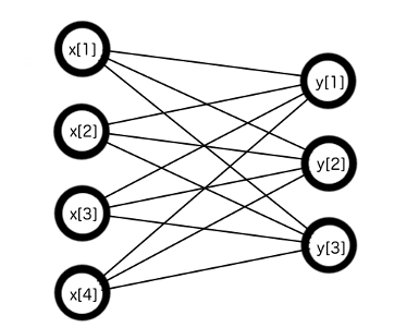
A fully-connected feedforward layer consists of a bunch of neurons (also called perceptrons), each of which is connected to every input of the layer.
More precisely, a fully-connected layer accepts \(M\) floating point numbers as inputs, and outputs \(N\) floating point numbers, where \(N\) is the number of neurons in the layer. We imagine each of the neurons to be connected to each of the \(M\) inputs by an edge. For each edge, there is a corresponding parameter \(\theta[m,n]\) (here \(1 \leq m \leq M,\ 1 \leq n \leq N\)) that can be trained.
Let \(x[m]\) denote the input elements and \(y[n]\) denote the output elements.
Forward pass. For each neuron, we compute the output as the inner product $$ y[n] = \sum_{i=1}^M \theta[m,n] \, x[m] $$ Intuitively, the trained parameter \(\theta[m,n]\) regulate the influence of the mth input on the nth output.
Backward pass. Let \(L\) denote the loss function. Suppose that \(\displaystyle \frac{\partial L}{\partial y[n]}\) is known for each n. We would like to compute \(\displaystyle \frac{\partial L}{\partial \theta[m,n]}\) for gradient descent and \(\displaystyle \frac{\partial L}{\partial x[m]}\) for the previous layer.
Derivatives with respect to weights (Info for gradient descent) Using the chain rule, we have the useful decomposition $$ \begin{align*} \frac{\partial L}{\partial \theta[m,n]} &= \sum_{n'=1}^N \frac{\partial L}{\partial y[n']} \frac{\partial y[n']}{\partial \theta[m,n]} \\ &= \frac{\partial L}{\partial y[n]} x[m] \end{align*} $$
Derivatives with respect to inputs (Info for backpass) Using the chain rule again, we have the decomposition $$ \begin{align*} \frac{\partial L}{\partial x[m]} &= \sum_{n=1}^N \frac{\partial L}{\partial y[n]} \frac{\partial y[n]}{\partial x[m]} \\ &= \sum_{n=1}^N \frac{\partial L}{\partial y[n]} \theta[m,n] \end{align*} $$
Each output of the fully-connected layer is put through a nonlinear function. This is important to enable the neural network to be able to approximate arbitrary continuous functions. Since a composition of two linear functions is again a linear function (and similarly for affine functions), without doing this, a neural network would only be able to fit linear (or affine) functions.
The original choice of nonlinearity was a step function, which had an interpretation as a ``gate'' that could either turn the neuron on or off. This was later replaced by smoother logistic nonlinearities (or hyperbolic tangents). The current standard seems to be ReLU (rectified linear unit) and its variants (leaky ReLU, MaxOut, ...), which is a step back to a step function. ReLU has the following forward and backward passes:
Forward pass. For each input \(x[m]\), compute the output as \( y[m] = \max(0, x[m])\). (There are as many outputs as inputs.)
Backward pass Assume \(\displaystyle \frac{\partial L}{\partial y[m]}\) are known. Then almost everywhere \( \displaystyle \frac{\partial L}{\partial x[m]} = \frac{\partial L}{\partial y[m]} \frac{\partial y[m]}{\partial x[m]} = \frac{\partial L}{\partial y[m]} \cdot 1_{x[m]>0}\). Because the ReLU has no adjustable parameters, this is all the information required for the backward pass.
Fully-connected neural networks with a softmax head is the best family of classifiers so far. They outperform kNN on data sets of the same size, are faster in time-per-classification, and take up less memory.
The following plots show the improvement in classification accuracy as a fully-connected network with two hidden layers (16,382x128x128x16 nodes, where the input and output layers are included) is trained for 256 epochs. The training set size is 32,768. For each deformation type, the training hyperparameters are \(\alpha = 0.005,\ \lambda=0.001\), with a minibatch size of 32. The blue curve indicates accuracy on the training set and the green curve accuracy on a test set of 1024 images.| Low deformation | Med deformation | High deformation |
| Low deformation | Med deformation | High deformation |
| Number of nodes in hidden layers |
128x128 | 128x128x128 | 1024x1024 |
|---|---|---|---|
| Legend:
Yellow: Low
Blue: Med
Purple: High
|
Viewing a neural network as a computational graph, (classical) convolutional nets introduce two new types of layers (which can be viewed as types of new graph nodes): convolutional layers and pooling layers. In general, convolutional layers make sense for dimensions of any input, but here I will describe only two-dimensional inputs (this is the typical case for image classification).
A (2D) convolutional layer accepts as input a finite collection of floating point numbers indexed by the set \(I \times J \times K\), where \(I, J\) are linearly-ordered, \(|I|\) can be thought of as image width in pixels, and \(|J|\) as image height in pixels. For \(K\), it is typical to have \(K = \{R,G,B\}\) in the input layer (for the three color channels), and for further layers to have \(K\) index the filters of the previous layer (if the previous layer was also convolutional).
The convolutional layer moves an input window (that is typically smaller than the full image) across the image, in order to learn local features.
A convolutional layer takes the following four additional parameters as input:
(More generally, one can imagine specifying different widths and strides for each input dimension.)
We expand \(I\) and \(J\) by \(p\) elements at each end, but keep using the notation \(I \times J \times K\) for the index set of the padded input.
The tunable parameters of the layer are the weights \(w_{k'}[a,b,c]\), where \(0 \leq a \leq w-1,\ 0 \leq b \leq w-1,\ 0 \leq c \leq \left|K\right|-1\), and \(0 \leq k' \leq n-1\). There is a weight attached to each pixel of the input window, for each slice. The same weights are used for each position of the input window, which is known as weight-sharing. The weights are to be tuned using gradient descent, with the gradients of the loss function with respect to the weights computed by back-propagation.
The output is a finite collection of floating point numbers indexed by the set \(I' \times J' \times K'\), where
Let \(x[i,j,k]\) denote the elements of the input and \(y[i',j',k']\) denote the elements of the output.
Forward pass. For each index \((i',j',k') \in I' \times J' \times K'\), set \(i_0 = i' \cdot s\) and \(j_0 = j' \cdot s\). These are the coordinates of the ``upper-right corner of the input window''. Then $$ y[i',j',k'] = \sum_{a = 0}^{w-1} \sum_{b=0}^{w-1} \sum_{c=0}^{|K|-1} w_{k'}[a,b,c]\, x[i_0+a,j_0+b,c] $$ Note: We do not include a non-linearity as part of the definition of a convolutional layer. Typically one wants to place one, for example a ReLU layer, right after.
Back pass. Let \(L\) denote the loss function. As usual, we suppose that the derivatives \(\displaystyle \frac{\partial L}{\partial y[i',j',k']}\) are known, and would like to compute \( \displaystyle \frac{\partial L}{\partial w_{k'}[a,b,c]}\) for gradient descent and \( \displaystyle \frac{\partial L}{\partial x[i,j,k]}\) for back-propagation to the previous layer.
Derivatives with respect to the weights (Info for gradient descent). The Chain Rule gives the usual useful decomposition $$ \frac{\partial L}{\partial w_{k'}[a,b,c]} = \sum_{i',j'} \frac{\partial L}{\partial y[i',j',k']} \frac{\partial y[i',j',k']}{\partial w_{k'}[a,b,c]} $$ From the definition of \(y[i',j',k']\) in the forward pass paragraph, we see that $$ \frac{\partial y[i',j',k']}{\partial w_{k'}[a,b,c]} = x[i'\cdot s + a,\, j'\cdot s + b,\, c]$$ and consequently $$ \frac{\partial L}{\partial w_{k'}[a,b,c]} = \sum_{i',j'} \frac{\partial L}{\partial y[i',j',k']}\ x[i' \cdot s + a,\ j' \cdot s + b,\ c] $$
Derivatives with respect to the node values (Info for back-propagation). Similarly, the Chain Rule gives the useful decomposition $$ \frac{\partial L}{\partial x[i,j,k]} = \sum_{i',j',k'} \frac{\partial L}{\partial y[i',j',k']} \frac{\partial y[i',j',k']}{\partial x[i,j,k]}$$ We see that $$ \frac{\partial y[i',j',k']}{\partial x[i,j,k]} = w_{k'}[i-i' \cdot s,\ j - j' \cdot s,\ k] \cdot 1_{\substack{0 \leq i - i' \cdot s < w\\ 0 \leq j - j' \cdot s < w}} $$ and so \begin{align*} \frac{\partial L}{\partial x[i,j,k]} &= \sum_{i',j',k'} \frac{\partial L}{\partial y[i',j',k']} w_{k'}[i-i'\cdot s,\ j - j' \cdot s,\ k] \cdot 1_{\substack{0 \leq i - i'\cdot s < w \\ 0 \leq j - j' \cdot s < w}} \\ &= \sum_{k' = 0}^{n-1} \sum_{i' = \lceil (i-w+1)/s \rceil}^{i' = \lfloor i/s \rfloor} \sum_{j' = \lceil (j-w+1)/s \rceil}^{j' = \lfloor j/s \rfloor} \frac{\partial L}{\partial y[i',j',k']} \, w_{k'}[i - i' \cdot s,\, j - j' \cdot s, k] \end{align*} The padding should be undone before passing to the previous layer.
It may be worthwhile to record two special cases of the above update:
When \(s=w\). We have \(\displaystyle \left\lceil \frac{i-w+1}{s} \right\rceil = \left\lceil \frac{i+1}{s} \right\rceil - 1 = \left\lfloor \frac{i}{s} \right\rfloor\). Therefore, the sum in \(i'\) contains just one term, and similarly for the sum in \(j'\). We have, in this case, therefore, that $$ \frac{\partial L}{\partial x[i,j,k]} = \sum_{k'=0}^{n-1} \frac{\partial L}{\partial y\left[ \left\lfloor i/s \right\rfloor, \left\lfloor j/s \right\rfloor, k' \right]} \, w_{k'}[i^*,\ j^*,\ k] $$
There are several types of possible pooling layers, but I have implemented only maxpooling. Intuitively, the purpose of the pooling operation is to make the classifier more invariant to small and local perturbations of the image.
Similarly to a convolutional layer, a maxpool layer accepts a collection of floating point numbers indexed by the set \(I \times J \times K\) as input, and produces a collection of floating point numbers \(I' \times J' \times K'\) as output.
The following additional parameters are required to determine the layer:
The output dimensions depend on the input dimensions as follows:
Forward pass. For each index \((i', j', k') \in I' \times J' \times K'\), set \(i_0 = i' \cdot s,\ j_0 = j' \cdot s\). Then $$ y[i',j',k'] = \max_{ \substack{ 0 \leq a < w \\ 0 \leq b < w} } x[i_0+a,j_0+b,k'] $$ The output is taken to be the largest value in the input window.
Backward pass. Assume \(\displaystyle \frac{\partial L}{\partial y[i',j',k']}\) are known. For each \((i,j,k,i',j',k') \in I \times J \times K \times I' \times J' \times K'\), let $$ \begin{align*} \Delta(i,j,k,i',j',k') &= \begin{cases} 1, & x[i,j,k] \mbox{ is max input in window specified by } (i',j',k') \\ 0, & \mbox{otherwise} \end{cases} \\ &= \begin{cases} 1, & x[i,j,k] = \max_{\substack{ 0 \leq a < w \\ 0 \leq b < w }} x[i' \cdot s + a, j' \cdot s + b, k] \mbox{ and } k=k' \\ 0, & \mbox{otherwise} \end{cases} \end{align*} $$ Then, $$ \begin{align*} \frac{\partial L}{\partial x[i,j,k]} &= \sum_{i',j',k'} \frac{\partial L}{\partial y[i',j',k']} \frac{\partial y[i',j',k']}{\partial x[i,j,k]} \\ &= \sum_{i',j',k'} \frac{\partial L}{\partial y[i',j',k']} \Delta(i,j,k,i',j',k') \end{align*} $$ (Strictly speaking the max function is not everywhere differentiable, but in practice the set where it isn't is sparse enough that it can be ignored.)
In practice, the window stride is usually chosen to be equal to the window width. In this case, only one summand remains in the above sum. It is efficient to keep track of the index of the max input during the forward pass, and then use it in the backpass.
Since a maxpool layer has no trainable parameters, this is all of the information that is necessary for the backward pass.
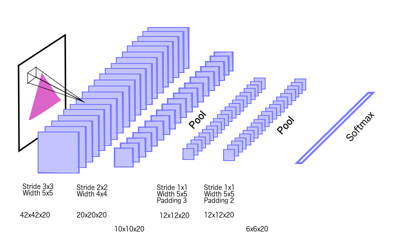
There are very many parameters to play with, and I stopped at using two architectures (one is smaller and one is larger)
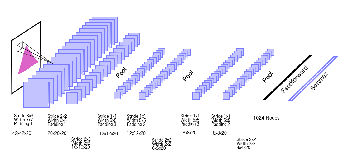
Convolutional neural networks perform the best out of the classifiers I tried on my problem. Convolutional networks are also among the best performers on the most difficult present day benchmarks --- most of the classifiers that perform the best on ImageNet as of September 2020 are versions of ResNets, which are Convolutional neural networks combined with several additional techniques that simplify training deeper networks (residual connections, and batch normalization).
The following plots show classification accuracy on a test set of 1024 images as a function of the number of training epochs. The blue curve shows the accuracy on the training set, and the green curve accuracy on the test set.
The plots below are for the small network. The hyperparameters were: \( \alpha = 0.0025,\ \lambda = 0.00025\), with a minibatch size of 32 and training size of 65,536.| Low deformation | Med deformation | High deformation |
| Low deformation | Med deformation | High deformation |
Obtaining a plot of best attained accuracy as a function of training set size is more difficult, because convolutional networks appear to be more sensitive to hyperparameter settings (so that the same hyperparameters do not work well across a cross-section of different training set sizes).