One of the leading Neural Network architectures in Computer Vision is that of Residual Neural Networks (ResNets).
As of October 2020, most of the entries on the ImageNet classification leaderboard are ResNets combined with algorithms for choosing particularly effective ResNet architectures (each of these algorithms goes by its own name: among others, there are EfficientNets, FixEfficientNets, RegNets, LambdaResNets). A recent paper (An Image is Worth 16x16 Words: Transformers for Image Recognition at Scale) reports comparable results for a Transformer architecture, so perhaps this situation will soon change and ResNets will be supplanted by Transformers in vision (however, at the moment this is unclear because training the Vision Transformer is more expensive than training ResNets).
ResNets were introduced by He, Zheng, Ren, and Sun (Deep Residual Learning for Image Recognition) in 2015. Roughly speaking, "ResNets = ConvNets + Residual Connections" (that is, ResNets are obtained by adding skip/residual connections to the list of architectural elements that are available for designing a usual Convolutional Neural Network). He and his coauthors motivate the introduction of residual connections by observing that as the depth of a ConvNet without residual connections (that the authors call a plain ConvNet) increases, beginning at a certain depth and thereon, the top accuracy achieved by the classifier tends to degrade (or, the desired accuracy levels are not reached in feasible time). This is surprising, because a deeper network has the capacity to completely mimic a shallower network, by simply having some of the layers act as the identity function. The idea of adding residual connections is to make the default operation of the neural network the identity function, with the learned behaviour of the network describing deviations from the identity. So, He and coauthors introduce an inductive bias towards the network performing the identity operation, by means of adding residual connections to the network. This idea has proven to be quite effective and ResNets do continue to improve with increasing depth.
Residual connections turn out to be useful more generally: for example, they are used in Transformers and (somewhat anachronistically and arguably) in LSTMs, among many other architectures.
Very deep neural networks take quite a lot of computation to train. A collection of techniques for making training faster and more efficient by reusing previously trained models goes under the name of Transfer Learning. One flavour of Transfer Learning is to train deep and expensive networks once, then use them as fixed feature extractors (meaning, roughly, functions that transform the input data into a collection of features that form a better representation of the data) for multiple problems. For example, instead of retraining a very deep network anew for every application, one uses a pre-trained ResNet (or another network) on ImageNet (or another dataset) as a fixed feature-extractor, and trains a relatively shallow network attached to the output of the feature-extractor ResNet. Another flavour of Transfer Learning is to train the entire network (in the example, the base ResNet, together with the smaller classifier head), but use a much lower learning rate for the base ResNet than for the classifier head (so as to preserve the learned features, but "fine-tune" the extractor to the present problem). One can also imagine various combinations of these two approaches.
There are several ResNet architectures available in PyTorch Vision: ResNet-18, ResNet-34, ResNet-50, ResNet-101, ResNet-152 (the numeric suffix gives the number of layers in the network). Optionally, one can load each of these networks with parameters that have been pre-trained on ImageNet. Here, I would like to compare the accuracy of a plain ConvNet to that of a MNIST or CIFAR-10 classifier with a ResNet base. It turns out that the pre-trained versions available in PyTorch are not quite the same as the networks described in the ResNets paper, so one cannot use them to replicate the results of the paper. However, the results are comparable to those in the paper (if one wished to replicate the results in the paper, that is possible by specifying the architecture described in the paper manually).
CIFAR-10 is one of the standard datasets for benchmarking image classification models. It consists of 60,000 3x32x32 images grouped into ten categories of 6,000 images each. The training set consists of 50,000 images, and the test set consists of 10,000 images.
Here is the link to the complete script on GitHub (the script name is resnet.py) for setting up a CIFAR-10 classifier with a (optionally pre-trained) ResNet base in PyTorch. The script is relatively simple and consists of the following parts:
It is necessary to import the following modules:
Loading and setting up CIFAR-10:
Defining the network and the forward pass:
Setting up the optimizer and the learning rate scheduler:
The training and testing follow the usual format for PyTorch. To save some space here, I do not include them, but please see the complete script (the script name is resnet.py) if needed.
It is difficult to make a comparison of the best results each network can attain, because optimal hyperparameter settings can change network-to-network. I ended up comparing the best results attained by each network, after 20 epochs of training, with a minibatch size of 32, and three possible learning rate schedules: "Fixed" means that the parameters of the ResNet base were frozen and the ResNet was used as a fixed feature extractor; "Tuned" means that the ResNet base was trained with a lower learning rate than the head (described in the code snippet above: base starts at 0.001 and head starts at 0.1, both are multiplied by 0.1 after 10 epochs); "Trained" means that both the base and the head were trained with the same learning rate (beginning at 0.1 and switching to 0.01 after 10 epochs). With these conditions, the best performance by far was attained by the "Tuned" approach on pre-trained nets. It is possible that the "Trained" approach can reach the same results with different hyperparameters and more training, but it is not clear that this has any advantage over tuning, which is faster and attains great results.
(I do not expect that either Fixing or Tuning a ResNet that was initialized with random weights will give particularly good results, but it is still important to test this out to be sure that it is the pre-training that makes the difference.)
Classification accuracy of ResNets (clicking on the radio buttons next to the classification results will display the corresponding graphs of loss and accuracy over training):
The last rows provide information on how several simpler networks perform on CIFAR-10, for some additional context. The first among them is the classification accuracy attained by just the head layer, without passing the data through the base ResNet first. The performance is much worse, only attaining 55% accuracy (I found that this was the case even when trying to train the classifier head for 100 epochs). The architecture used for ConvNet-2n pastes the block (Conv->BatchNorm->ReLU->Conv->BatchNorm->ReLU->MaxPool) n times, followed by a feedforward layer of 1024 nodes, and a linear layer for the ten CIFAR-10 classes.
For comparison, in the 2015 ResNets paper, ResNet-20 achieved 91.25% accuracy, ResNet-56 achieved 93.03% accuracy, and ResNet-110 achieved 93.57% accuracy. The architectures of these networks are different from those of the PyTorch ResNets (the ones the appear in the paper use fewer parameters), but if a rough comparison by similar depth is made, the pre-trained (and tuned) PyTorch ResNets outdo the results reported in the paper on CIFAR-10. The best current result on the CIFAR-10 classification leaderboard is 99.5% accuracy, which is only 2.5 percent better that the best result attained with a tuned ResNet 152 (that was pre-trained on ImageNet).
MNIST is a data set for the task of recognizing hand-written digits. It is another standard data set for testing Image Classification systems. MNIST consists of 60,000 training examples and 10,000 test examples. MNIST is considered to be simpler task than CIFAR-10, and even logistic regression approaches 90% accuracy, so ResNets aren't necessary to do well. However, MNIST is still a useful benchmark.
Much of the code can be reused to test out ResNets on MNIST. The data set is already implemented in PyTorch Vision:
One subtlety is that a PyTorch ResNet expects an input of size 3x224x224, whereas MNIST is grayscale and only uses a single color channel. The first layer of the ResNet can be modified to take 1x224x224 images as follows:
I still upsampled the MNIST images to 224x224, since otherwise they would get collapsed to single pixels in the ResNet convolutional layers.
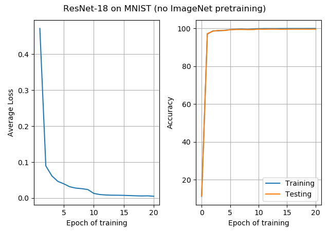
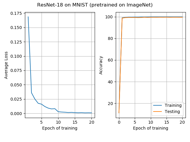
The results for ResNet-18: As expected, MNIST is a simpler task than CIFAR-10. Both pre-trained and non-pre-trained nets attain 99.6% accuracy, very quickly. The pre-trained ResNet achieved this accuracy a little faster.
One of the leading Neural Network architectures in Natural Language Processing is that of Transformers.
Similar to ResNets, Transformers employed in practice tend to be very deep, and take a long time to train. The idea of Transfer Learning is correspondingly also commonly applied with transformers, such as OpenAI's GPT-n, or Google's BERT.