GitHub page for this project.
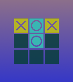
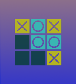
To learn a bit about reinforcement learning, I implemented several agents for playing 3x3 Tic-Tac-Toe. The agents are: Minimax, a non-learning rules-based agent that I named Heuribot, an agent trained using Tabular Q-learning, and a DQN agent. The result is the following program:
| Algorithm: | Play as: | |
(The front-end is written in Javascript, but the actions of the agents are decided based on table lookup from the output of another program written in C++.)
I found that implementing agents for playing Tic-Tac-Toe is a fairly good way to dip a toe into reinforcement learning. The problem is not quite trivial, but small enough that experiments are fast. More specifically, the following features of Tic-Tac-Toe are agreeable for playing around with reinforcement learning: (1) Tic-Tac-Toe is a small game (it has only 5,478 valid board states, with at most nine valid actions per state); (2) Tic-Tac-Toe is a solved game, always ending in a tie in optimal play, and it is not difficult to implement non-learning optimal (meaning never losing in regular play) agents to test the learning agents against, which is helpful for evaluation of the learning agents; (3) Tic-Tac-Toe is a commonly-played game, which makes the results simpler to explain to others.
On the negative side, Tic-Tac-Toe is well-explored. Looking through some textbooks after beginning this project, I found that often Tic-Tac-Toe came up in the examples or exercises --- for example, Tic-Tac-Toe appears in the first chapter of Reinforcement Learning: An Introduction, 2nd ed., by Sutton and Barto, and in the exercises to the first chapter of Machine Learning by Mitchell. It seems unlikely that anything new can be said in connection with Tic-Tac-Toe. Every agent explored here got to optimal play (in the sense of never losing), without requiring me to come up with novel techniques or ideas (altough some of them (especially DQN) took quite a bit of effort to get working well).
The following two pages contain evaluations of every board position (up to symmetry) by the four agents:
(To set down a bit of terminology: I will refer to the players of the game as agents (as commonly done in reinforcement learning), or simply players. Agents will take turns placing Xs and Os on the game board. I will refer to the X and O symbols as marks. The board is divided into nine cells, and there are eight lines comprised of three cells each (three horizontal lines, three vertical lines, and two diagonals). The cells are categorized into four corner cells, four side cells, and a single centre cell, in the evident way. A player wins by being the first to fill one of the lines entirely with their marks. A fork is a position in which the opponent has two overlapping lines with two of the cells of each line filled with their mark, and the remaining cell of the line blank; if a player forks their opponent, they have a sure way to win on their next turn.
By the game graph I will mean the rooted directed acyclic graph, where nodes are in one-to-one correspondence with valid board positions, the root node is the empty board, and there a directed edge between a pair of boards if one can pass from one to the other by placing a valid mark. By a terminal node or leaf node of the graph, I will mean a node with no outgoing edges.)
Minimax is a standard algorithm for implementing agents for two-player turn-based finite zero-sum games (some examples of such games are chess, go, checkers, and many others, including Tic-Tac-Toe and its variants). Minimax is an effective algorithm, especially when the game is small enough that the entire game tree can be stored in memory, and plays optimally against an optimal opponent. As the game size grows, it soon becomes necessary to combine Minimax with heuristic evaluation rules, since it becomes practically infeasible to search large subgraphs of the game graph (which full Minimax requires at the initial stages of the game). However, the game graph for 3x3 Tic-Tac-Toe is small enough that this is unnecessary.
Roughly speaking, the Minimax algorithm is based on the following principle --- the move a player should make is the one that leads to the best possible outcome for the player, assuming that the move made in response by their opponent is also a move that leads to the best possible outcome for the opponent.
The best-possible outcome from a given position is represented by a real number called the utility of that position. Then, the goals of the two players are translated into opposing utility-optimization problems: the goal of one of the players is taken to be that of reaching the outcome with the highest-possible utility, and the goal of their opponent is taken to be that of reaching the outcome with the lowest-possible utility. I will assume hereafter that in Tic-Tac-Toe X is the maximizing player.
The utilities of the leaf nodes are defined based on the corresponding game position. For example, every leaf of the Tic-Tac-Toe game graph is either a win for X, a win for O, or a tie. By convention, these options are often assigned the utilities of +1, -1, and 0, respectively.
Then, the utilities of the various nodes of the game graph are assigned recursively, by starting with the leaves (terminal nodes) and propagating up through the DAG. The propagation is done as follows: for a board position in which X is to move, the utility of that position is taken by definition to be the maximum of the utilities of its children (that is the best possible outcome for X); for a board position in which O is to move, the utility is taken to be the minimum of the utilities of its children. (Effectively, this way of computing utilities enables the Minimax agent to do a look-ahead search just by looking at the utilities of the moves immediately available to it.)
When the game graph is too large, one can still run a version of the Minimax algorithm, but since the leaf nodes are not accessible in reasonable time, one uses approximate (heuristically-evaluated) utilities of the positions at a certain depth away from the current position, then propagates the utilities up in a recursive manner, as before.
Having the notion of utility in-hand, we can now formally state the Minimax principle as follows: suppose that the game is in state \(s\), with a set of available actions \(A_s\). The player X is to move. For each possible action \(a \in A_s\), denote the resulting state \(s'(a)\), and for each response \(a' \in A_{s'(a)}\), let \(s''(a,a')\) denote the resulting state.
Since we are assuming that O moves to its best-available outcome from state \(s'(a)\), the utility of state \(s'(a)\) will be equal to $$ \underset{a'}{\operatorname{min}} u(s''(a,a'))$$ Therefore, the move leading to the best possible outcome for X is $$ \underset{a}{\operatorname{argmax}} \min_{a'} u(s''(a,a')). $$ Symmetrically, the best outcome for O, assuming that X plays its best-possible outcome, is $$ \underset{a}{\operatorname{argmin}} \max_{a'} u(s''(a,a')). $$
The following is a small example of the propagation of the utilities from the terminal nodes up through the game graph. The numbers in the parentheses are obtained by following the recursive procedure outlined above.
| |||||||||||||||||||||||||||||||||||||||||||
| \( \swarrow \) | \( \downarrow \) | \( \searrow \) | |||||||||||||||||||||||||||||||||||||||||
|
|
| |||||||||||||||||||||||||||||||||||||||||
| \( \swarrow \) | \( \searrow\) | \(\swarrow\) | \(\searrow\) | ||||||||||||||||||||||||||||||||||||||||
|
|
|
| ||||||||||||||||||||||||||||||||||||||||
| \(\downarrow\) | \(\searrow\) | \(\swarrow\) | \(\downarrow\) | ||||||||||||||||||||||||||||||||||||||||
|
|
|
| Find-Utility (node, player) |
|
if node is terminal return utility assigned to node else if player is the maximizing player max for each child of node Find-Utility(child, min) return maximal child utility else // player is the minimizing player min for each child of node Find-Utility(child, max) return minimal child utility |
Once the utilities are known, the Minimax players move greedily (X to a node with the highest-available utility, O to the node with the lowest-available utility).
For another baseline, I constructed a non-learning Tic-Tac-Toe player that uses heuristic rules to evaluate the board position and decide on its best possible move. I named this agent the Heuribot.
Already for a game as simple as Tic-Tac-Toe, a fair number of rules are necessary to obtain an agent that plays anywhere close to optimally (by this I mean that, at least, the agent does not lose from any position that allows for a tie or victory). One appreciates that for problems of larger scale, this approach can become unwieldy.
The collection of heuristics that I ended up using is a slight modification of the approach described in the article Flexible Strategy Use in Young Children's Tic-Tac-Toe by Crowley and Siegler (I found this reference through wikipedia). Most of these heuristics (which are described in more detail below) are quite intuitive, and perhaps I should not have deprived myself of the fun of formulating them for myself, but I wanted to spend the time required to do so on other parts of this project, since the main point was for me to learn something about learning agents!
Heuribot makes the first possible move out of the following hierarchy (in the following, by a ``line'' I mean any horizontal row, vertical row, or diagonal):
| Win | If there is a line with two of Heuribot's marks, and one blank, the Heuribot completes the line to win. |
| Block the Opponent's Win | If there is a line with two of the Heuribot's opponent's marks, and one empty cell, Heuribot places its mark in the empty cell of the line, blocking the opponent's victory. |
| Fork | If the Heuribot can fork, it does so. |
| Block an Only Fork | If the opponent can make a fork on their next turn, and every opponent's fork can be blocked by placing a single mark, Heuribot places that mark. |
| Force the Opponent to Block | If there is a line with one of Heuribot's marks, and two blanks, the Heuribot considers placing a second mark in that line to force the opponent to block. To decide whether or not to place the mark, the Heuribot conjecturally traces through the sequence of forced moves caused by placing the mark, until either the first non-forced move or the end of the game is reached. If the sequence of forced moves ends with the end of the game, and Heuribot wins at the end of the sequence, it places the mark; if the Heuribot loses, it does not place the mark. Otherwise, the Heuribot counts the number of ways the opponent can create a fork at the end of the sequence. If it is Heuribot's turn at the end of the sequence of forced moves, Heuribot accepts the move if the opponent can make at most one fork (because the Heuribot can block that fork); if it is the opponent's turn, the Heuribot only accepts the move if the opponent cannot create a fork. |
| Play the Centre | If the centre is blank, Heuribot places its mark in the center. |
| Play an Opposite Corner | If a corner is occupied by an opponent's mark, and the opposite corner is blank, the Heuribot places its mark in the opposite corner. |
| Play an Empty Corner | If there is a blank corner, the Heuribot places its mark there. |
| Play an Empty Side | If there is a blank side, the Heuribot places its mark there. |
A funny detail regarding the strategy described in the Crowley-Siegler article is that if you play the bot against itself, the X side will win 100% of the games. This is certainly not optimal (to be fair to the authors of the article, they do not claim that their bot is optimal). The trouble is with an underspecification of the following rule:
Block Fork
If there are two intersecting rows, columns, or diagonals with one of my opponent's pieces and two blanks, and if the intersecting space is empty, then
If there is an empty location that creates a two-in-a-row for me (thus forcing my opponent to block rather than fork), then move to the location. Otherwise, move to the intersection space (thus occupying the position that the opponent could use to fork).
|
\( \rightarrow \) |
|
\( \rightarrow \) |
|
\( \rightarrow \) |
|
\( \rightarrow \) |
|
|||||||||||||||||||||||||||||||||||||||||||||
| X opens in the center | O responds in a corner | X plays in the opposite corner | O attempts to avoid X's fork by forcing X to block | X makes the forced move, but still forks O | |||||||||||||||||||||||||||||||||||||||||||||||||
What is missing from the Crowley and Siegler strategy is a rule for deciding between multiple ways of forcing the opponent to block, if such exist. We surely do not want to make the above play, where X is forced into obtaining a fork (and hence winning). For this example, O is better off forcing X to block by moving into the upper-right corner instead of the upper side of the board. Similarly, moves that force the opponent to block into completing three-in-a-row should be avoided.
When following the strategy described by the above hierarchy, the Heuribot is good enough to never lose. Sometimes, however, the Heuribot has trouble telling apart moves that are guaranteed to win as opposed to ones that will merely tie (against an opponent that forces the tie when it has the chance). I find Minimax to be a subtler judge of the quality of a position, which is not surprising as the utility assignment algorithm effectively enables Minimax to be able to look ahead to the terminal nodes.
As a side-product of implementing the Heuribot, I also obtained a position-classifier (each game position can classified by the best possible move that can be made from the position according to Heuribot), which can help in evaluating the other agents.
The following matrix summarizes how the three players match up against each other. The numbers are proportions of games won by the respective agent (or tied), out of 100,000,000 games, rounded to three places after the decimal. The first move of each player is not randomized, so that, for example, the minimax X player always uses the same opening.
| X Minimax | X Heuribot | X Random | |||||||||||||||||||
|---|---|---|---|---|---|---|---|---|---|---|---|---|---|---|---|---|---|---|---|---|---|
| O Minimax |
|
|
|
||||||||||||||||||
| O Heuribot |
|
|
|
||||||||||||||||||
| O Random |
|
|
|
The minimax and heuribot players are fairly evenly matched. One interesting observation from the comparison table is that neither heuribot nor minimax quite manage to win every game against the random opponent, allowing some ties even when playing as X. This agrees with my intuition, because, for any sequence of moves made by a player (even a player following a best-possible strategy), there exists a sequence of moves made by the opponent that will tie the game. Because there are finitely many states, there should be a nonzero probability that the random agent will discover a tieing sequence of moves. It seems that this probability is somewhere around 0.005, if the first move is not randomized (the reason I am mentioning the latter explicitly is that I will care about randomizing the first move later on). It would be interesting to explicitly bound the probability of a random opponent tieing a game against any possible agent, but I have not done so.
Going by the comparison table alone, the Minimax agent and the Heuribot agent are fairly similar. The gameplay of the agents has some distinctive characteristics, however, and it may be worth looking for other evaluations that more clearly tell them apart. Having more evaluations will help to obtain a better picture of the learned agents later on as well.
Perhaps the most effective way of comparing the agents is simply to study their evaluations of all of the possible board states. A table of such evaluations (with boards that are similar by a reflection or rotation identified together) can be found on the following pages:
By design, minimax tends to be quite defensive, because it looks to minimize its opponent's gains. Moreover, by our choice of utility function, the minimax player does not distinguish between rewards in the near- versus long-term (of course, for Tic-Tac-Toe the difference between near- and long- term is just a few moves). In particular, minimax may not take the victory on turns when it is set up to win, or even choose moves that cause it to tie instead of win (in situations when its opponents play suboptimally and bring the game to a situation when minimax has a chance to win).
The following is an example of a position that is not played by minimax as efficiently as it could have been (the utility of a terminal position is computed as +1 for a win and -1 for a loss (and 0 for a tie), minimax is playing as O):
In this example, minimax wins on the next move (it has set up a fork, and it wins if it goes to the left side or the bottom side), and this is the reason why the move that was made is evaluated as being of equal utility as the move that wins immediately.
This suggests looking at how average game length varies from agent to agent (measured in total number of turns a game takes). This will be a number between five and nine, inclusive.
The results for the baseline agents are summarized in the following table. It is only worth recording the results against the random opponent of course, because minimax and heuribot always tie each other, so the games between the two are always nine turns long. The numbers record proportions of games of the given length, out of 100,000,000 played. Only the nonzero proportions are recorded.
| Minimax | Heuribot | |
|---|---|---|
| Random playing as O | 5 turns: 0.370 7 turns: 0.516 9 turns: 0.112 |
5 turns: 0.799 7 turns: 0.167 9 turns: 0.035 |
| Random playing as X | 6 turns: 0.419 8 turns: 0.387 9 turns: 0.194 |
6 turns: 0.775 8 turns: 0.108 9 turns: 0.117 |
The minimax player can be adjusted to play more aggressively by adding a small penalty to the utility for each additional mark the agent places down. One way to do this is to compute the utility as (10 - Number of filled squares) for an X win, and -(10 - Number of filled squares) for an O win.
I will be trying to teach the players to play from a randomized initial position (meaning that X's opening is made randomly before the agent is allowed to choose their move). The following two tables summarize the results of every possible pairwise match-up, with the X player being allowed to choose their first move, and with the first move of the game randomized. As before, they are computed by playing 100,000,000 games.
The interesting data is in the rows and columns that involve the Random agent. Every other matchup always ends in a tie!
| X Minimax | X Heuribot | X Random | X Tabular Q | X DQN | |||||||||||||||||||||||||||||||
|---|---|---|---|---|---|---|---|---|---|---|---|---|---|---|---|---|---|---|---|---|---|---|---|---|---|---|---|---|---|---|---|---|---|---|---|
| O Minimax |
|
|
|
|
|
||||||||||||||||||||||||||||||
| O Heuribot |
|
|
|
|
|
||||||||||||||||||||||||||||||
| O Random |
|
|
|
|
|
||||||||||||||||||||||||||||||
| O Tabular Q |
|
|
|
|
|
||||||||||||||||||||||||||||||
| O DQN |
|
|
|
|
|
The numbers for the Tabular Q-learning agent in the above tables are fairly stable (different training runs yield nearly equal numbers; the numbers above are the best among several training runs, but the variance is not large). The agent is a Double Tabular Q-learning agent that is trained by self-play for 3,000,000 games. The hyperparameters are: \(\alpha\) begins at 1, and is multiplied by 0.9 at regular intervals throughout training (this is done 100 times, and \(0.9^{100} \approx 0.00003\)); \(\epsilon\) begins at 1 and is regularly annealed by 0.1 until reaching 0.1 by the time a third of the training games are finished, and left at 0.1 from thereon; \(\gamma = 0.999\) throughout training.
Similarly, the numbers of the DQN agent are fairly stable (but it is necessary to keep track of the best performance during training, since the training may not end having converged on the best agent). The training parameters are described in the DQN section.
For the rest of this page, I will describe the Q-learning agents in greater detail.The standard formal setting for Reinforcement Learning is the theory of Markov Decision Processes. I include a short summary of the basics here, for the purpose of sketching the motivation for the Q-learning algorithm, referring to the book of Sutton and Barto for a more detailed exposition.
The RL problem is represented as a collection \(S\) of states. For each possible state, there is an associated collection \(A_s\) of possible actions. An action takes the agent from a state s to another state s' (often, in a nondeterministic way, so the action yields a probability distribution over \(S\) instead of a single state s'), and has an associated reward r. An episode / trajectory / realization of an MDP starting at state \(s_0\) is a discrete sequence \((s_0, a_0, r_0; s_1, a_1, r_1; \dots)\), where \(a_i\) is an action taken in state \(s_i\) that brings the agent to state \(s_{i+1}\), and has an associated reward \(r_i\).
For simplicity (this is sufficient for Tic-Tac-Toe), we assume that the sets of possible states, actions, and rewards are finite. To each state \(s\) and action \(a\), there is a corresponding transition probability \(p(s', r| s, a)\), which is required to satisfy the Markov property.
The goal of the agent starting at \(s_0\) is to maximize its discounted reward \( Reward = r_0 + \gamma r_1 + \gamma^2 r_2 + \cdots \), where \( 0 \leq \gamma \leq 1\) is the discounting factor, which is a hyperparameter. Discounting adds an additional degree of freedom in specifying the problem, but also is a technical device that allows one to deal with possibly infinite trajectories. There are other reward schemes that are studied in place of discounted rewards, but I will not go into them here.
A policy is a function on the set of all possible states \(S\) that specifies a choice of action for every state, or possibly a probability distribution over the set of possible actions from that state. Let \(\pi\) be a policy. For each state s and action a from s, define \(Q_\pi (s,a) = E_\pi[ Reward | s_0 = s, a_0 = a]\), then define the optimal Q-function as \(Q^*(s,a) = \max_{\pi} Q_\pi(s,a)\). Given an optimal Q-function \(Q^*\), there is a policy \(\pi_*\) so that \(Q^* = Q_{\pi_*}\). Any such \(\pi_*\) is called an optimal policy.
It can be proven that if, given a policy \(\pi\), we define a new policy \(\pi'\) by $$ \pi'(s) = \operatorname{argmax}_{a \in A_s} Q_{\pi}(s,a) $$ Then \(Q_{\pi'}(s,a) \geq Q_{\pi}(s,a)\) for all pairs \((s,a)\). Moreover, if \(\pi\) is fixed by the above process, then \(\pi\) is an optimal policy. This provides a way of iteratively approximating an optimal policy using the Q-function, called policy-improvement.
Tabular Q-learning was introduced by C. Watkins in his 1989 PhD thesis (Watkins' sketch of a proof of convergence (under certain fairly mild hypotheses) that appeared in his thesis was completed by him and Dayan in 1992). The idea of Watkins' Q-learning algorithm is to modify the above algorithm to make it computationally less expensive, by replacing the actual value of \(Q_\pi(s,a)\) by an estimate coming from the Bellman equation.
Finally, one combines the above estimate with the idea of Temporal-Difference (TD) learning to make the method model-free.
We obtain the following update rule for Q: Initialize the Q-function approximation \(Q^0\) with small random numbers. Then, collect agent experience (in Tic-Tac-Toe, this means play the game), in the form of a sequence of tuples \((s_n, a_n, r_n, s_{n+1})\), where \(s_n\) is some state, \(a_n\) is an action taken from \(s_n\), bringing the agent to state \(s_{n+1}\), with associated reward \(r_n\), and this data is used to construct a sequence \(Q^0, Q^1, Q^2, \dots\) of approximations to \(Q^*\) by the update formula $$ Q^{n+1}(s,a) = (1-\alpha_n) Q^n(s,a) + \alpha_n \left( r_n + \gamma_n \max_{a' \in A_{s'}} Q^{n}(s',a') \right) $$ where \(0 \leq \alpha_n \leq 1\) is an additional sequence of hyperparameters, referred to as the learning rate sequence. Once an agent reaches a terminal state, it restarts from one of the initial states and continues training. A very nice feature of Q-learning is that the policy that is used to pick actions during training does not need to be the policy encoded by the Q*-function (or its approximations) --- for this reason, Q-learning is said to be an off-policy algorithm. This feature of Q-learning makes it possible to reuse collected data, which is useful when training data is expensive to obtain.
For Tic-Tac-Toe, the tabular Q-learning agent performs as well as minimax, and converges quite nicely! (Although some fiddling with the agent parameters was definitely required to get to this point.)
The hyperparameters involved in the training of the tabular Q-learning agent are
| Alpha \( \alpha \) | Learning rate |
| Gamma \( \gamma \) | Discount factor |
| Epsilon \( \epsilon \) (or a similar alternative, as in Boltzmann exploration) | Exploration rate |
I would like to explore how the characterisics of the learning agent depend on the choice of each of the hyperparameters. Strictly speaking, the hyperparameter effects may be correlated with one another, but to get a good understanding it will be enough to look at how the behaviour of the learning agent changes as a function of one of the hyperparameters, the others being fixed.
Learning Rate (\( \alpha \)). The learning rate is bounded below by 0 and above by 1. Intuitively (as may be seen from the update rule formula), the learning rate parametrizes how much individual updates affect the Q-values; there is a tradeoff between speed and stability of learning. A lower learning rate means slower, but more stable convergence; a higher learning rate means (possibly) faster convergence, but less stability. However, learning rates that are too low can get stuck in local minima.
The following plots are all made with \( \gamma = 0.9\) and \( \epsilon = 0.4 \). They are obtained by performing 10 training runs, each of which consists of 300,000 episodes against the random opponent, and computing the proportion of wins by the agent (playing as X) out of 10,000 games played, at regular intervals during training. The first move of the agent is randomized. The graph on the left displays each run in a different color, while the graph on the right displays the average of the runs (the points within the shaded region in the background are within a single standard deviation of the average).
The best values of \( \alpha\) seem to be 0.2 or 0.3, but the range from 0.1 to 0.4 seems reasonable. Already at \(\alpha = 0.4\), the high learning rate seems to begin to do damage to learning. The training periods start becoming more noisy, and the maximum of the agent's performance decreases. If the learning rate is initially set too low (\(\alpha = 0.01\) is one such example in the above plots), we also run into poorer performance.
Discount factor (\(\gamma\)). The discount factor is also bounded by 0 from below and by 1 from above. Intuitively, the discount factor specifies how much more the agent values short-term vs. long-term rewards.
The following plots are all made with \( \alpha = 0.1\) and \(\epsilon = 0.4\). They are now obtained by averaging 100 (not 10, to reduce variance, since I am no longer interested in plotting single training runs) training runs consisting of 300,000 training episodes (left) and 1,000,000 training episodes (right) against the random opponent each, for each value of \(\gamma\).
One may guess
that a Q-learning agent with low \(\gamma\) may prefer to end games sooner,
which leads us to consider the average length of a winning game as a function of \(\gamma\).
The conjecture is indeed true, and
the results are summarized in the following table. Each of these agents was
a Single Q-learning agent trained from scratch over 2,000,000 games,
with \(\alpha\) and \(\epsilon\) following the annealing schedules described earlier (after the overall summary).
In the plot, red corresponds to games of length 5, green games of length 7, and blue games of length 9.
Gamma
0.0
0.1
0.2
0.3
0.4
0.5
0.6
0.7
0.8
0.9
1.0
Overall win proportion
0.888
0.990
0.991
0.990
0.990
0.987
0.990
0.984
0.984
0.984
0.984
Win proportion at depth 5
0.509
0.833
0.833
0.822
0.822
0.787
0.787
0.729
0.729
0.694
0.380
Win proportion at depth 7
0.300
0.149
0.153
0.162
0.161
0.183
0.191
0.233
0.232
0.262
0.512
Win proportion at depth 9
0.079
0.007
0.005
0.006
0.008
0.017
0.012
0.022
0.023
0.028
0.092
Exploration rate (\(\epsilon\)). If the training steps of the agent are chosen follows the simple policy of taking the action that maximizes the Q-value over all actions that are possible to undertake in the agent's current state, there is a danger of the agent settling into a local maximum game, and playing that game over and over for the remainder of training. Therefore, it is advantageous to sometimes take actions that appear to be suboptimal, in hopes of finding a better policy, if such exists. The exploration parameter controls how frequently such exploratory actions are undertaken.
The following plots are made with \(\alpha=0.1\) and \(\gamma=0.9\).Although not displayed in the above plots, with \(\epsilon=0\), the agent does tend to stay in a suboptimal policy.
Removing noise and instabilities at the tail by gradually decreasing \(\alpha\) and \(\epsilon\) The Q-learning agent gets to a good level of play relatively quickly (it tends to become good enough to always tie against Minimax within 30,000 games of training). With more training, the agent even gets to the 0.995 win rate against Random (when playing as X, and when free to decide on its first move). However, if the hyperparameters are kept constant, the agent tends not to stay at the optimum, getting slightly bumped off its peak at random intervals, no matter how many episodes it is trained for. Why doesn't this contradict the convergence theorem?
In fact, in the precise statement of Watkins' convergence theorem, there are some additional assumptions about the learning rate. One way of informally thinking about these additional assumptions is that they require that \(\alpha\) tends to 0, but not too fast. In theoretical work on Q-learning, the following state-dependent learning rates are used frequently: a record of the number of times \(n(s)\) each state \(s\) has been visited is kept throughout training, and the learning rate is taken to be a suitable decreasing function of \(n(s)\), for example \(\alpha(s) = 1/n(s)\). These learning rates satisfy the hypotheses of Watkins' theorem.
In practice, I found that the following ad-hoc approach to scaling down the learning rate worked well enough (and in fact better than the learning rates described in the previous paragraph): the training starts with \(\alpha = 1,\ \epsilon = 1\), then \(\alpha\) is multiplied by 0.9 at intervals of ((total episodes)/100), so that by the end of training \( \alpha = 0.9^{100} \approx 0.00003 \), and \(\epsilon\) is decreased by 0.1 at regular intervals down to \(\epsilon = 0.1\) by the ((total episodes)/3), and equal to 0.1 from thereon.
The problem recognized by Double Q-learning is that max is a biased estimator. A slight modification of the Q-learning algorithm (which is described in C. Sutton's free online book) improves the state of affairs.
In my tests, the performance of the Double Q-learned agent does tend to be better than, or at least comparable to, the performance of a Single Q-learned agent, and, as expected, Double Q-learning does tend to converge faster. The plots show the progress of the agents as they train by self-play. In each of the plots, the agents are playing as X against the indicated opponent. The first move is randomized in all of the games.
Interestingly, against the random opponent the Double-Q agent dips below the Q agent slightly. This seems to be an artifact of self-play (if the Double-Q agent playing as X is trained against the Random opponent playing as O, the Double-Q agent in fact catches up to the 0.991 win rate we see for the Single Q-learning agent, and avoids the dip we see for the Single Q-agent). For the match-ups involving Q-learning opponents, they were both pre-trained on 5,000,000 games and fixed for all of the tests. There is another interesting consequence of self-play (at least this is the way I understand this observation) in the plots of the games of the Q-learning agents against each other. Namely, since the agents are trained by playing against themselves, they become particularly good opponents for themselves; so, the agents progress more slowly against their own counterpart (for example, Single Q-learning learns to play against Single Q-learning more slowly than does Double Q-learning, and vice versa!).
For each of the plots, the hyperparameters were \(\gamma = 0.9\), \(\alpha\) = 1 decaying down to 0.9100, \(\epsilon\) = 1 decaying down to 0.1 by the time a third of training was finished. The plots display the mean over 50 training runs, with the shaded area behind the plot representing a single standard deviation.
|
Display plot of (playing as X): Versus: (playing as O) |
|
The basic idea of a DQN (Deep Q-Network) is to use a deep artificial neural network to approximate the \(Q^*\)-value function of a reinforcement learning agent. So, very roughly speaking, the slogan is ``DQN = Q-learning + Deep neural nets''. The DQN approach loses the nice convergence guarantees that Q-learning had, but can be applied to problems of much higher scale. The first success of DQN was learning to play many Atari games fairly well, with no input beyond the pixels of the last four game frames, and with a single set of hyperparameters for all of the games. The state space of Atari games is large enough that the naive tabular approach to Q-learning becomes infeasible.
The idea of applying a function approximator to the Q*-function did not originate with the DQN paper. Approached naively, however, using an artificial neural network for this purpose tends to be very noisy. The major contribution of the DQN authors was in proposing a collection of tricks that help to stabilize training; the two major tricks are: using a second network that updates more sporadically than the training network as an update target, and using an experience replay buffer. These tricks remove a few of the sources of correlation from the training data, taking advantage of the fact that a Q-learning agent can be trained off-policy. In trying to implement an agent that did not apply these ideas, I found that the entire network tended to fill up with NaNs after some time, usually just short of finishing training. More subtly, even if the network did not blow up, the noisy behaviour of the approximation interfered with learning, to the point where the agents peaked quite far from optimal play (with a win rate of around 0.80 against the random opponent in the best cases, and usually worse).
Because Q-learning worked so well for Tic-Tac-Toe, and DQN is a kind of approximation of that process, there is perhaps less motivation for writing a DQN Tic-Tac-Toe agent. However, I now had some context for Tic-Tac-Toe from writing the other agents, and the relatively simple and familiar setting let me focus on understanding and implementing the DQN techniques. It was also interesting to compare the behaviour of the approximator with the thing being approximated.
DQN was introduced in the conference paper Playing Atari with Deep Reinforcement Learning, which was expanded to the paper Human-level control through deep reinforcement learning, both by Vlad Mnih with many coauthors (the first one with 7 authors, and the second with 19 authors).
Notation: Let \(\theta\) denote the parameters of the approximator of the Q-value function. For DQN, the approximator will typically be a neural network, and \(\theta\) in this case denotes the trained weights of the network. For any state-action pair \((s,a)\), let \(Q_\theta(s,a)\) denote the output of the approximator evaluated at the tuple \((s,a)\); for a neural network, this typically means that the representation of state \(s\) is fed into the network as the input, and the value of the output node corresponding to the state obtained after taking action \(a\) is read from the output.
The original Atari DQN paper used a neural network architecture that involved convolutional layers, which are common to applications that involve vision. Although there is a decidedly visual element to the Tic-Tac-Toe board, because convolutional layers are computationally expensive to train, and because the problem is so simple, I decided to limit the network to several relatively small feedforward hidden layers.
I chose to work with the naive board representation, where the input and output layers both have 9 nodes, each representing a cell of the game board. Inputs of 1, -1 and 0, represent an X mark, O mark, and no mark, respectively.
After a lot of experimentation, the network architecture I decided on is:
The following architectural choices seem to be particularly important:
At the bottom of this page, I included several plots to help demonstrate some of the comments collected in the above list.
The last two hyperparameters in the list, namely the replay buffer size and target update frequency, are specific to DQN. I will now describe them.
Speaking intuitively, a major source of instability for training a neural network to fit the Q-value function is that moves from the same run or round are not statistically independent. So consecutive moves from the same run of a game make the network overfit to that run. This may be less of an issue for Tic-Tac-Toe because the games are so short, but DQN is meant to handle games of much larger scope, where the same run may last for hundreds, thousands, or more, updates.
The DQN paper introduced several tricks to improve the stability of training:
Instead of training live, the idea is to take advantage of the fact that the Q-learning may be done off-policy (meaning that the agent does not have to follow the policy encoded by the Q-function to get the next update). As the agent is trained, the agent plays according to the policy encoded by the current approximate Q-values (meaning takes moves that maximize \(Q_\theta\)). The agent's play history is stored in a cache of tuples \((s, a, r, s')\), where s is the current state, a is the action the agent takes, r is the agent receives, and s' is the next state (the size of this cache is another hyperparameter, typically it is in the hundreds of thousands). Then, after each move, a minibatch of previous moves is randomly sampled from the cache (according to some scheme, the simplest being uniform random sampling, but there are more sophisticated techniques such as Prioritized Experience Replay), and the network is updated by taking an SGD step that minimizes the following loss: $$ \text{Loss} = \frac{1}{2} \sum_{(s_b, a_b, r_b, s'_b) \in \text{Minibatch}} \left( Q_\theta (s_b, a_b) - \gamma \left( r_b + \max_{a'_b \in A_{s'_b}} Q_\theta (s'_b, a'_b) \right) \right)^2 $$ where by definition \(Q_\theta(s,a) = 0\) for all terminal states \(s\) (actually, it is not quite SGD, because the term that's multiplied by \(\gamma\) is treated as being constant with respect to \(\theta\) --- this will actually become true below when the target network is introduced).
Intuitively, the random sampling should help to disentangle the correlations between moves from the same training run, because we are now looking at snippets of different runs in the same minibatch. Each training run can now be learned from multiple times as well, which improves the data efficiency of the method.
Another source of instability is that in the above expression for the loss, the same neural network is used to evaluate the current approximation of the Q function and the proposed update. Speaking intutively, one can imagine that this can have some undesirable feedback effects on training.
A proposed workaround is to introduce a second network that is updated more sporadically (meaning not every minibatch). The first network is called the trainer network, and the sporadically-updated network is called the target network. Periodically, the target network is set to be equal to the trainer network; how frequently the second network updates is another hyperparameter. Denoting the Q-function approximation produced by this network by \(\widehat{Q}_\theta\), the expression for the loss now becomes
$$ \text{Loss} = \frac{1}{2} \sum_{(s_b, a_b, r_b, s'_b) \in \text{Minibatch}} \left( Q_\theta (s_b, a_b) - \gamma \left( r_b + \max_{a'_b \in A_{s'_b}} \widehat{Q}_\theta (s'_b, a'_b) \right) \right)^2 $$As discovered by the person who invented Double Tabular Q-learning (Hado van Hasselt), this also can be combined nicely with the idea of Double Q-learning: we now use the target network to select the best action from state \(s'\), and the trainer network to evaluate the Q-value: $$ \text{Loss} = \frac{1}{2} \sum_{(s_b, a_b, r_b, s'_b) \in \text{Minibatch}} \left( Q_\theta (s_b, a_b) - \gamma \left( r_b + Q_\theta (s'_b, \operatorname{argmax}_{a'} \widehat{Q}_\theta(s'_b, a'_b)) \right) \right)^2 $$
To avoid exploding gradients, cut off the updates at -1 and 1. This can be interpreted as using the Huber Loss instead of the Mean-Squared Error Loss.
Optimizer. The following plots all use a 9x32x32x9 feedforward network (to reduce training time), but the remaining parameters are the same as listed above (except the optimizers) --- the minibatch size is 2. The differences in performance are dramatic. One can argue that the hyperparameters have been tuned for Adam and not the other optimizers, but even after trying to fine-tune for the other optimizers they perform worse. Because DQN has quite a high variance between training runs, two plots of different training runs are included for each optimizer (the training takes too long to take an average among more training runs than two for the purposes of these plots).
| Two runs with Adam | Two runs with plain SGD | ||
|---|---|---|---|
| Two runs with SGD + Momentum | Two runs with RMSProp | ||
Minibatch. Continuing with a 9x32x32x9 feedforward network, the following plots show runs with various minibatch sizes (all with Adam).
| Two runs with Minibatch = 1 | Two runs with Minibatch = 8 | ||
|---|---|---|---|
| Two runs with Minibatch = 16 | Two runs with Minibatch = 32 | ||
Nodes in hidden layers. Plots made with Adam and minibatch size 2.
| Two runs with 8x8 | Two runs with 16x16 | ||
|---|---|---|---|
| Two runs with 64x64 | Two runs with 128x128 | ||
Varying the target update frequency. Plots made with Adam, 9x32x32x9 feedforward net, and minibatch size 2.
| Two runs with update frequency 1 | Two runs with update frequency 100 | ||
|---|---|---|---|
| Two runs with update frequency 1,000 | Two runs with update frequency 10,000 | ||
Varying the buffer size. Plots made with Adam, 9x32x32x9 feedforward net, and minibatch size 2.
| Two runs with buffer size 25,000 | Two runs with buffer size 50,000 | ||
|---|---|---|---|
| Two runs with buffer size 100,000 | Two runs with buffer size 300,000 | ||